Kickstarting ML Apps with Streamlit in 30 Minutes

This blog post is the first in our two-part series about Streamlit. If already mastered the basics of Streamlit head over to our second article on how to Build Streamlit apps with State

How to go from idea to interactive machine-learning web app before your coffee gets cold.

1 Why Streamlit?

When you’re validating an AI idea you want to iterate, not integrate. Streamlit is a one-file, zero-config framework that turns a Python script into a shareable web app instantly—no templates, routing, or front-end build systems in sight.

Because of that low ceremony, it shines as a proof-of-concept (PoC) launcher: tweak data, swap models, hit Save, and the browser hot-reloads. Stakeholders see progress in real time while you stay firmly in your ML comfort zone.

Streamlit also comes with:

• Built-in widgets (sliders, select boxes, file upload) that require no JS.
• Reactive layouts that rebuild only the parts affected by user input.
• Caching primitives to keep expensive data loads and model inits snappy.

Ready to get started? Follow the tutorial below to build the app. We’ve published the app on the Streamlit Community Cloud for you to play around. Find the repo and dive into the code on GitHub.

2 Our Use Case: Penguins 🐧

We will build a penguin species classifier. The Palmer Penguins data set (in seaborn) includes bill length/width, flipper length, body mass and the island each bird calls home. Good variety, clean structure, no ethical minefields.

⚠️ Heads up!
This post is not a machine learning tutorial. We won’t dive into the theory behind data splitting, model training, or evaluation.
Instead, the focus is on Streamlit — and how it lets Machine Learning Engineers stay in their zone of genius (building models) without getting lost in frontend code. 🛠️➡️🤖

3 The App, Line by Line

3.0 Install the goodies

pip install streamlit scikit-learn pandas seaborn matplotlib

Create app.py and follow along.

# ── 0. Setup: import the usual suspects ──
import streamlit as st      # 🔤️  Web UI in pure Python
import pandas as pd         # 📊  Data wrangling
import seaborn as sns       # 🐧  Penguin dataset helper
from sklearn.model_selection import train_test_split  # 🔀 Train/test split
from sklearn.preprocessing import StandardScaler      # ⚖️  Feature scaling
from sklearn.linear_model import LogisticRegression   # 🤖  Classifier
from sklearn.metrics import accuracy_score            # 🕏  Metric

3.1 Data loading (cached)

Load the data with the provided function, and add explanations in markdown for the users of the app.

📜 st.markdown(), st.subheader() and st.header()

These are your go-to tools for adding formatted text and section headers—Markdown-powered and refreshingly readable. They’re perfect for narrative flow, and unlike print(), they actually look good.

🧠 @st.cache_data

Used in load_data(), this memoizes expensive operations like data fetching or preprocessing. It’s a performance cheat code—subsequent reruns don’t reload unless the code or inputs change.

# ── 1. Dataset Overview ──
st.markdown("""
### 🐧 About the Dataset
The **Palmer Penguins** dataset is a popular alternative to the Iris dataset for beginner ML tasks. It records measurements for three penguin species (*Adélie*, *Gentoo*, and *Chinstrap*) from three islands in Antarctica.

**Key features:**
- `bill_length_mm`: Length of the penguin's beak
- `bill_depth_mm`: Depth/thickness of the beak
- `flipper_length_mm`: Flipper length (important for swimming)
- `body_mass_g`: Body weight
- `island`: One of three islands (categorical)
- `species`: Target label (what we want to predict)

We'll use only the numeric measurements to keep it simple.
""")

@st.cache_data
def load_data():
    # 1⃣ Load & drop missing rows for simplicity
    penguins = sns.load_dataset("penguins").dropna()

    # 2⃣ Encode the categorical target so scikit-learn is happy
    species_map = {s: i for i, s in enumerate(penguins["species"].unique())}
    penguins["species_id"] = penguins["species"].map(species_map)
    return penguins, species_map

penguins, species_map = load_data()

st.markdown("### 📟 Sample of the dataset")
st.dataframe(penguins.head())

st.markdown("---")
st.markdown("### 📈 Explore feature distributions")

# Define number of bins for histograms
NUM_BINS = 30

for feature in ["bill_length_mm", "bill_depth_mm", "flipper_length_mm", "body_mass_g"]:
    st.subheader(f"Distribution of {feature} by species")

    # 1. Create bins for the feature
    # We use pd.cut to divide the range of the feature into NUM_BINS intervals
    penguins[f'{feature}_bin'] = pd.cut(penguins[feature], bins=NUM_BINS)

    # 2. Group by bin and species, then count occurrences
    chart_data = penguins.groupby([f'{feature}_bin', 'species']).size().unstack(fill_value=0)

    # 3. Optional: Make bin labels more readable (e.g., "32.1-33.0")
    chart_data.index = chart_data.index.map(lambda interval: f"{interval.left:.1f}-{interval.right:.1f}")

    # 4. Display the data using Streamlit's native bar chart
    st.bar_chart(chart_data)

    # Clean up the temporary bin column (optional)
    penguins = penguins.drop(columns=[f'{feature}_bin']) # Keep if needed later

3.2 🧰 Sidebar widgets

Add some widgets to the sidebar so that users can configure the parameters for the model training.

• st.sidebar.header() – Adds a title to the sidebar.
• st.sidebar.multiselect() – Lets users pick multiple features (columns) to use for modeling.
• st.sidebar.slider() – Slidable widget to choose a numeric value (test/train split here).

# ── 2. Sidebar ──
st.sidebar.header("⚙️ Model settings")

features = st.sidebar.multiselect(
    "Choose features",
    [c for c in penguins.columns if penguins[c].dtype != "object" and c != "species_id"],
    default=["bill_length_mm", "bill_depth_mm", "flipper_length_mm", "body_mass_g"],
    help="Tick the boxes to include/exclude measurements."
)

test_size = st.sidebar.slider(
    "Test size (fraction of rows)", 0.1, 0.5, 0.2, 0.05,
    help="0.2 means 20% of the data will be unseen during training."
)

3.3 Training button + state magic

Copy the this code to train the ML model. The model will run at the press of a st.button

🟢 st.button() + st.session_state Buttons don’t just trigger actions—they can manipulate persistent session data like train_clicks or hold your model/scaler objects. session_state feels like global state.

# ── 3. Train & evaluate ──
if "train_clicks" not in st.session_state:
    st.session_state.train_clicks = 0

X = penguins[features]
y = penguins["species_id"]

if st.button("🚀 Train model", help="Fit a Logistic Regression on the selected features"):
    st.session_state.train_clicks += 1

    X_train, X_test, y_train, y_test = train_test_split(
        X, y, test_size=test_size, random_state=42, stratify=y)

    scaler = StandardScaler().fit(X_train)

    model = LogisticRegression(max_iter=200)
    model.fit(scaler.transform(X_train), y_train)

    preds = model.predict(scaler.transform(X_test))
    acc = accuracy_score(y_test, preds)

    st.success(f"Accuracy on unseen data: {acc:.2%} (run #{st.session_state.train_clicks})")

    st.session_state.model = model
    st.session_state.scaler = scaler

    with st.expander("What did we just do?", expanded=False):
        st.markdown("""
        1. **Split** the data so we don't cheat.
        2. **Scale** features – many models assume comparable numeric ranges.
        3. **Fit** Logistic Regression – a baseline linear classifier.
        4. **Score** on the 20% test set to approximate real-world performance.
        """)

3.4 Live prediction widget

🔢 st.number_input()

Used for live prediction inputs. It auto-generates labeled, bounded input widgets based on the range you give it. Sliders would’ve worked too, but number inputs give finer control for numerical values. Instant validation, no parsing needed.

🧱 st.columns() — Side-by-Side Layout You’re splitting the horizontal space into two equal columns (col1 and col2). Any widget placed inside with col1: will appear in the left half, and anything inside with col2: appears in the right half—like a grid system, but native to Python.

• Groups related inputs visually.
• Keeps the interface compact and readable.
• Gives you control over layout without writing CSS or HTML.

# ── 4. Interactive prediction ──
st.subheader("🔍 Try it out")

col1, col2 = st.columns(2)
with col1:
    bill_length = st.number_input("Bill length (mm)", min_value=30.0, max_value=60.0, value=45.0, step=0.1)
    bill_depth  = st.number_input("Bill depth (mm)",  min_value=13.0, max_value=22.0, value=17.0, step=0.1)
with col2:
    flipper     = st.number_input("Flipper length (mm)", min_value=170.0, max_value=240.0, value=200.0, step=1.0)
    mass        = st.number_input("Body mass (g)",      min_value=2500.0, max_value=6500.0, value=4200.0, step=100.0)

if st.button("Predict species"):
    if "model" not in st.session_state:
        st.warning("Train the model first! 🚦")
    else:
        sample = pd.DataFrame([[bill_length, bill_depth, flipper, mass]], columns=features)
        scaled = st.session_state.scaler.transform(sample)
        pred_id = st.session_state.model.predict(scaled)[0]
        pred_species = {v: k for k, v in species_map.items()}[pred_id]
        st.info(f"🧬 Likely species: **{pred_species}**")

        with st.expander("What does this mean?", expanded=False):
            st.write("""The model projects your inputs into the same scaled space it was
            trained on and outputs the most probable species label. 👈
            Remember: it's only as good as the data it has seen!""")

3.5 Quick EDA charts

Let’s display some charts to inspect the data interactively.

# ── 5. Quick exploratory chart ──
st.markdown("### 🔍 Feature interactions") st.markdown("Let's visualize how some features vary across species to understand which ones may be useful for classification.")

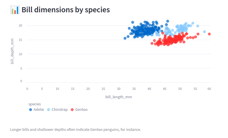
st.subheader("📊 Bill dimensions by species")
chart_data = penguins[["bill_length_mm", "bill_depth_mm", "species"]]
st.scatter_chart(chart_data, x="bill_length_mm", y="bill_depth_mm", color="species")
st.caption("Longer bills and shallower depths often indicate Gentoo penguins, for instance.")

4 Run and Have Fun

streamlit run app.py

That’s all there is to it. Your browser pops open; tweak sliders, train, predict. No Flask routes, no JavaScript build steps—just Python.

Now you can think about where to deploy your application. We deployed it for free on the Streamlit Community Cloud. All you need is to create an account on Streamlit and link it to your Github repo.

There are some other options to consider as well:

• Deploy it as a regular Python process in Docker
• Deploy it on any PaaS like Heroku or Azure.
• Create a space on Huggingface and use the option to deploy via streamlit directly.

TL;DR: Streamlit eliminates web friction so you can ship insights, not HTML. Penguins today; multimodal transformers tomorrow. Happy streaming!

This blog post is licensed under CC BY-SA 4.0