First steps with a graph database - using Python and ArangoDB

In this post we introduce the basics of a graph database and how to access it from Python. The database system used for storing and querying the data is ArangoDB, which was briefly described in a previous blog post. The Python driver of choice, as referenced in the official documentation, is Python-Arango; which can be accessed via its GitHub page.

Installation and set-up

For the purposes of this introduction, we installed the free and single instance Community Edition — which can be downloaded here — on a Linux (Ubuntu) machine. The instructions for installation via the package manager using apt-get can be found here. Upon successful completion of the installation, a server daemon can be launched via the command line by running:

arangod

This also starts a web interface that is reachable by default at localhost:8529 (see screenshot below). It is the most straightforward way to access server performance data, to perform administration tasks of databases, collections and users, as well as to query the data.

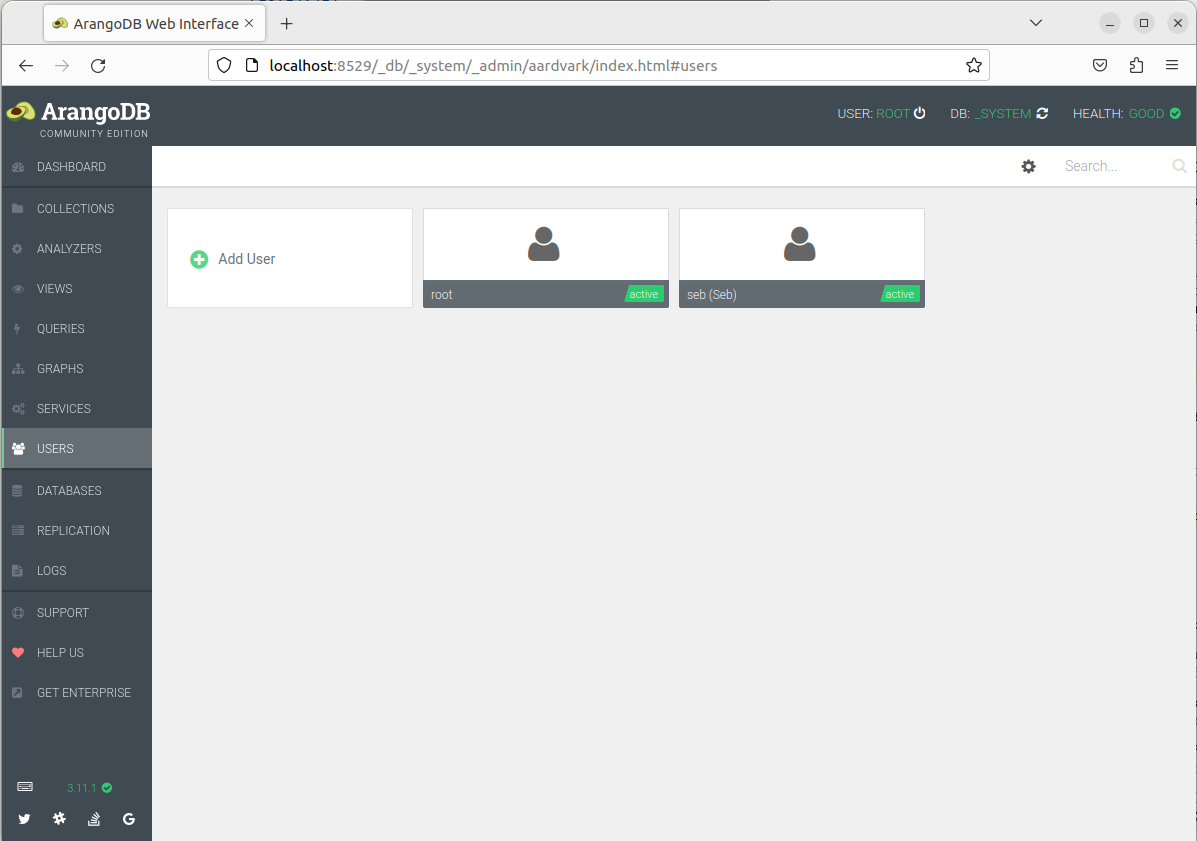
One database is automatically initialized, _system, which is accessible by the root user and cannot be deleted. It is the database one needs to connect to in order to create, delete or modify any other one. The active user and database can be seen in the top right corner of the web interface.

Connecting to ArangoDB from Python

As indicated above, Python-Arango is the official driver for database administration and data manipulation from within the Python ecosystem. Assuming we are already inside our python environment, we install the driver with:

python -m pip install python-arango

In the following code snippet, we connect to the _system database and perform some basic tasks.

# Load libraries
from arango import ArangoClient
from pprint import pprint # standard library for pretty printing

# Initialize some variables
client = ArangoClient(hosts='http://localhost:8529')
root_password = <YOUR PASSWORD FOR ROOT>
anna_password = <YOUR PASSWORD FOR ANNA>

# Connect to default database '_system' as 'root'
sys_db = client.db(
    '_system',
    username = 'root',
    password = root_password
   )

# Create new databases with two admin users
sys_db.create_database(
    name='test',
    users=[{'username': 'root', 'password': 'root_password'}, 
    {'username': 'anna', 'password': 'anna_password'}]
    )

sys_db.create_database(
    name='useless_db',
    users=[{'username': 'root', 'password': 'root_password'}, 
    {'username': 'anna', 'password': 'anna_password'}]
    )

# Delete database; any except for '_system'
sys_db.delete_database('useless_db')

# Retrieve list of all databases
sys_db.databases() 
# RETURNS 
['_system', 'test']

Elements of a graph database

The multi-model nature of ArangoDB influences the terminology about data records. The equivalent of tables and records in RDBMS are collections and documents, respectively. We can create and manipulate some empty collections as follows:

# Connect to 'test' database as user 'anna' 
test_db = client.db('test',
    username='anna',
    password=anna_password
    )

# Create collections
events_coll = test_db.create_collection(name='events')
assets_coll = test_db.create_collection(name='network_assets')
useless_coll = test_db.create_collection(name='useless_collection')
connections_coll = test_db.create_collection(
    name='connected_to', 
    edge=True
    )

# Delete collection
test_db.delete_collection(name='useless_collection')

# Retrieve list of all collections in current database
all_colls = test_db.collections()

The last command returns a list of dictionaries; one for each collection. Several system collections are automatically created, identified by the underscore prefix in their name. They are listed below by calling the value corresponding to their name attribute:

for i in range(len(all_colls)): 
    print(all_colls[i]['name'])
# RETURNS
_graphs
_aqlfunctions
_pregel_queries
_frontend
_apps
_queues
_analyzers
_fishbowl
_appbundles
_jobs
events
network_assets
connected_to

If we call one of the collections that we have just created, e.g. network_assets, we get the confirmation that it is not a system one, and we discover more key-value pairs:

# Pretty printing the contents of a collection
pprint(all_colls[-2])
# RETURNS
{'id': '211249',
 'name': 'network_assets',
 'status': 'loaded',
 'system': False,
 'type': 'document'}

Most attributes are self-explanatory but what about the type?

Collections of (vertex) documents

The default collection type is document, which stores data in JSON format. To understand the internal structure of documents, we start by populating one of our collections, like so:

# Insert documents manually into 'network_assets' collection
assets_coll.insert({'name': 'computer1',
    'ip': '192.168.1.1'})
assets_coll.insert({'name': 'computer2',
    'ip': '192.168.1.5'})
assets_coll.insert({'_key': '90210',
    'first_name': 'Beverly',
    'last_name': 'Hills',
    'age': 25})

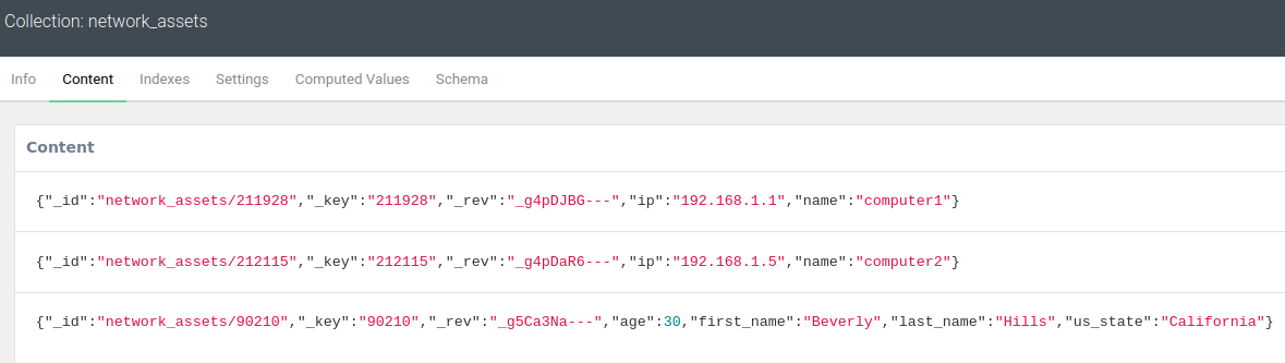
The contents can be displayed and modified from the web interface (see screenshot below). 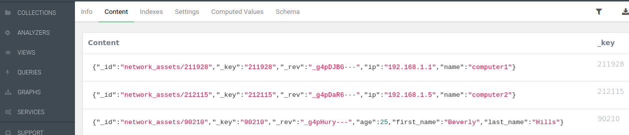Three default unique attributes are automatically created for every document:

• _key: unique identifier string. If no value is given at document creation, it will be created automatically
• _id: unique identifier string. Concatenation of collection name and _key
• _rev: unique alphanumeric string tracking all changes during the lifetime of a document

Schema validation

In the image above, the third document does not follow the same _key pattern as the others because it was explicitly given at data creation. Also, since by default no schema is being enforced in this NoSQL database system (briefly discussed in this previous post), the three documents can perfectly have very different data attributes.

Schema validation is straightforward to implement. In the section Schema (to the right of Computed Values in the screenshot), we write down our constraints in JSON Schema format; see step-by-step guide here.

Here is a suggestion for our network_assets:

{
  "message": "Schema validation error", 
  # what gets returned when inserting data not following the schema
  "level": "strict",
  "type": "json",
  "rule": {
    "properties": {
      "name": {
        "type": "string"
      }, # 'name' takes a string value
      "ip": {
        "type": "array",
        "items": {
          "type": "string"
        } # 'ip' takes a list of string values
      }
    },
    "required": [
      "name" # attribute is compulsory. 'ip' is not
    ],
    "additionalProperties": {
      "type": "string"
    # allows any other optional attributes, as string values
    }
  }
}

The .insert() operation would have failed for the Beverly Hills document because it did not contain any name attribute. The ip numbers in the other documents would not have been accepted either, because the schema requires a list instead of a single string value.

Collections of edge documents

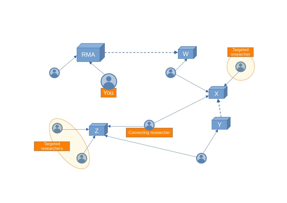
So far we have focused on documents that could be used as vertices, in other words the nodes in a graph representation; see the network graph below, from this article. But we saw in the second large block of code above that we could create an edge collection by passing True to the edge argument:

connections_coll = test_db.create_collection(
    name='connected_to', 
    edge=True
    )

In order to be usable as edges between vertices, in the upcoming Graphs section, a slightly different schema is being enforced by ArangoDB. Besides the _id, _key and _rev, that function like in vertex collections, we now have two additional compulsory attributes:

• _from: the _id of a source vertex
• _to: the _id of a destination vertex

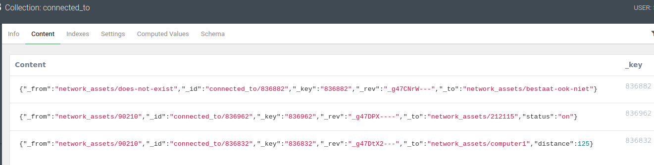
As for the first edge document above (the one with _key: 836882), the connected vertex documents need not exist in any collection. Or they could come from multiple collections, such as was implicitly the case in the network graph above. There, we would typically have a researchers collection and an organizations collection. The third edge document above does not point _to an existing vertex document either, because we have concatenated the collection network_assets and the name instead of the _key... Only the second edge document is between existing members of our network_assets collection.

The power of ArangoDB as a graph database lies in the flexibility it offers in terms of edge attributes. Not only can we characterize vertices by anything like their first name, (last) name, ip address, type, country, profession, asset category, ... that is relevant for the problem at hand, but we can also give any number of useful attributes to the edges themselves. In the screenshot above, we made use of a string value for the attribute status ("on") and an integer for the distance (125) between the respective vertices.

Graphs

The first thing we can do is to create a Named Graph — manually via the web interface or programmatically with the Python driver —, like our rather unimpressive test graph below, built from our network_assets vertices and our connected_to edges. 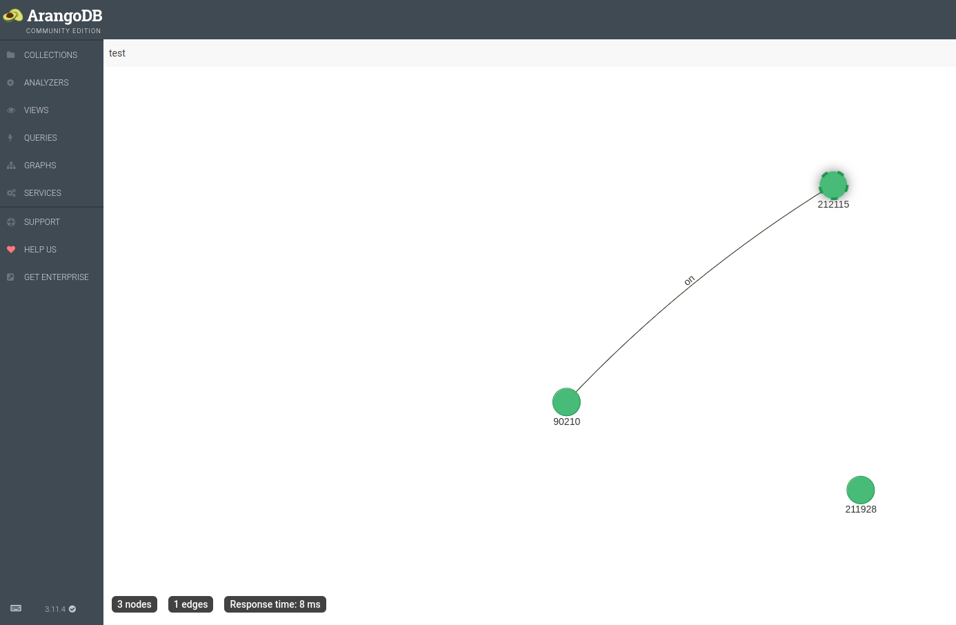By default, the graph view window displays the _key value for all the vertices. Here, we have changed the settings to also display the value of the status attribute for the edge(s); on, in this case. A Named Graph requires the following as input:

• one edge collection
• one or more _from vertex collection(s)
• one or more _to vertex collection(s)

This explains why our inexistent vertex documents do not appear: network_assets/does-not-exist, network_assets/bestaat-ook-niet, network_assets/computer1. This is also why network_assets/211928 appears in the graph view. Although it is not in our edge collection, it is loaded along with all of the vertex collection.

Graph queries or traversals

A more practical way to create a graph is by instructing ArangoDB to connect together, on the fly, all the relevant vertex documents (from multiple vertex collections, if needed) via one or multiple edge collections. For instance, here is a query with the Python-Arango driver that we can use to interrogate the graph behind the researchers-organizations network depicted above:

# Get all the possible connection pathways starting from <You>, 
# up to and including all <Targeted Researchers>
query = test_db.aql.execute('FOR researcher, work_connection, path \
  IN 2..7 ANY "researchers/you" rma_employees x_employees y_employees z_employees \
  OPTIONS { uniqueVertices: "path" } \
  FILTER IS_SAME_COLLECTION( "researchers", path.vertices[-1] ) \
  RETURN DISTINCT CONCAT_SEPARATOR( " -> ", path.vertices[*].name ) \
  ')

Let's break down the code line by line:

• in the AQL query executor, we initialize the variables that exist for the duration of the graph traversal: an iterator for researcher vertices (based on one or several vertex collections), one for the work connection edges (based on one or several edge collections) and one for the paths that are being traversed during the query execution (based on vertex-edge-vertex sequences that are only materialized in memory in the local context of the query). This is where a graph database stands out compared to an RDBMS, optimizing look-ups to start and remain only around the relevant vertices.
• we traverse from minimum 2 (MIN value is required) to maximum 7 (MAX value is optional) degrees of separation. We start at You and disregard the direction of the edges (ANY). OUTBOUND and INBOUND exist, but looking at the network figure above, we can see that in the researchers-organizations case, we are continuously traversing the graph along as well as opposite the arrow directions. As indicated above, here we can submit multiple edge collections (for RMA, X, Y, Z) in which the query executor will look for relevant _from — _to pairs.
• a typical graph database option is to avoid looping through certain vertex-edge-vertex combinations. Here we specify that, for any path from a start- to an end-vertex, we allow each vertex to occur only once.
• since we are interested in researchers and not organizations nodes, we only keep the paths that end ([-1] index) with a member of the researchers collection.
• we return the unique paths by writing the name value of each vertex (hence the [*] index), separated by the string " -> " for readability.

The query returns a Cursor object, which can either be iterated through in a for loop or by repeatedly calling the query.next() method until it is empty. Alternatively all of the Cursor output can be extracted in batch. The result is a Python deque, or double-ended queue; a list like container that is optimized for left and right appends and pops (see Python documentation). Depending on our goal with the output, we can for instance cast the deque as a Python set (not useful here since we used RETURN DISTINCT in AQL), as a simple list, or otherwise manipulate it, e.g. sort it:

pprint(sorted(query.batch())) # pretty print in Python the AQL output
# RETURNS
['you -> rma -> adam',
 'you -> rma -> w -> bob',
 'you -> rma -> w -> bob -> x -> charlie_targeted_researcher_1',
 'you -> rma -> w -> bob -> x -> eve',
 'you -> rma -> w -> bob -> x -> eve -> z -> dave',
 'you -> rma -> w -> bob -> x -> eve -> z -> florence_targeted_researcher_2',
 'you -> rma -> w -> bob -> x -> eve -> z -> geraldine_targeted_researcher_3',
 'you -> rma -> w -> bob -> x -> y -> dave']

CRUD operations

We already discussed how to Create documents earlier. An Update requires the document _key to be passed, along with any attribute that needs to be added or changed.

# Update an existing document
assets_coll.update({'_key': '90210',
  'us_state': 'California',
  'age': 30})

The updated attribute values for Beverly Hills can be seen below.

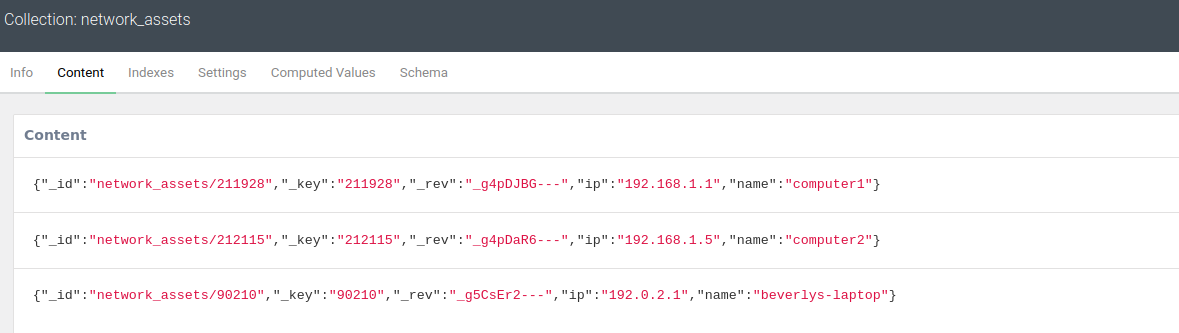
When we Replace a document, all existing attributes are overwritten. The document _key is again used as the unique identifier, and we need to provide zero or more attribute key-value pairs. Indeed, only the three default attributes are actually required: _id, _key, _rev.

# Replace all attributes of an existing document
assets_coll.replace({'_key': '90210',
  'name': 'beverlys-laptop',
  'ip': '192.0.2.1'})

The changes can be seen below:

Finally we can Delete a document with

assets_col.delete({'_key': '90210'})

This brings us to the end of our introduction to graph database concepts, having hopefully triggered some interest into the logical next step for exploration with ArangoDB and Python: network analysis and visualization.

This blog post is licensed under CC BY-SA 4.0