Guessing the width of an image

Interpreting a 1-D array of pixels is not possible by the human eye. And yet such data is available in several circumstances, like the dump of pixel arrays from RAM or disk, the availability of image files in RAW format (without the width) or when solving a Capture-The-Flag cybersecurity challenge with images.

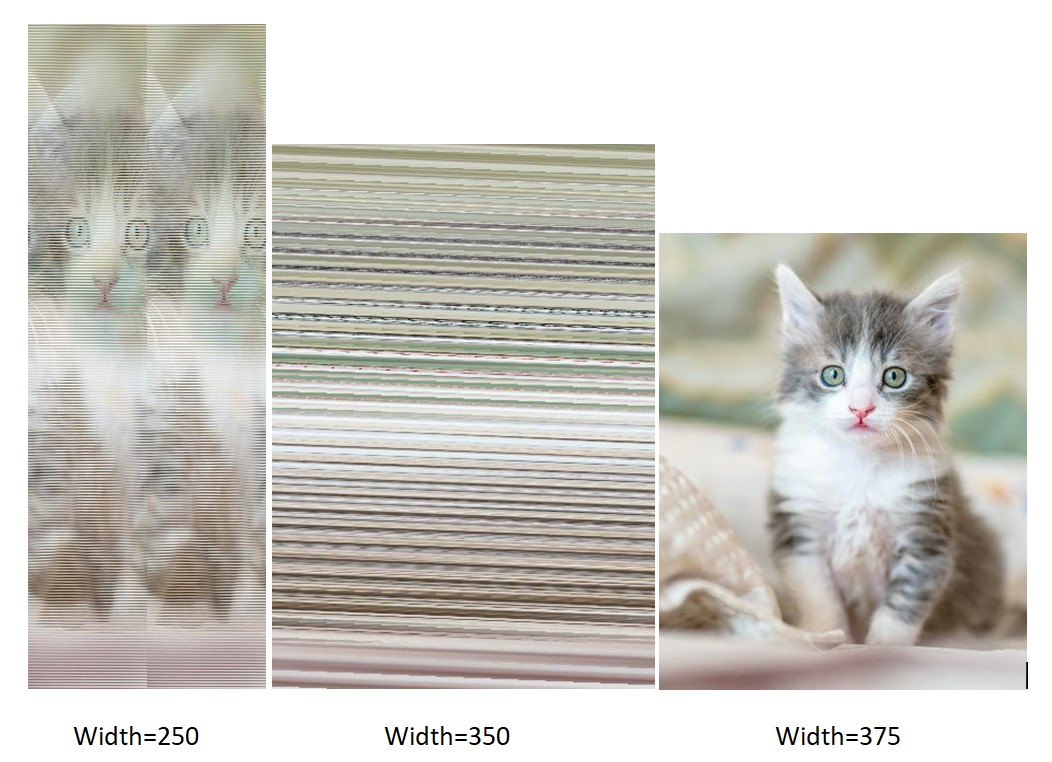
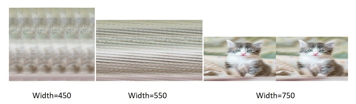Images with a wrong width may be difficult to interpret.

Guessing the appropriate width to form an intelligible image from a 1-D array necessitates a trial and error approach. The large number of pixels and the possibly large search space for the width requires image processing. And yet, reconstructed images with a value close to the right one may remain indistinguishable. Tuning the width parameter with visual evaluation may be heavy.

We propose in this blog an automatic procedure to find the correct original width of an image whose pixels are available as a 1-D array. The method is simple and efficient: it relies on the correlation between successive lines for a range of widths. It clearly highlights the correct width except for some images with strong periodic patterns or with poor image content.

1. Methodology

In most images and in particular for natural ones, the difference of intensity between neighboring pixels tends to be small due to correlation. If an image is not uniform, modifying the width parameter while keeping the same number of pixels (so, changing the height) will introduce discontinuities, for instance along vertical edges. If the image content is not periodic, one width will match consecutive rows the best.

The algorithm considers the pixel data as a 1-D array. Data can come from an image with correct or incorrect width or a 1-D list of pixel values. It computes a difference level from consecutive image rows for a range of width values.

The difference level is the Root Mean Square difference, that is the square root of the sum of the square of pixel intensity differences divided by the number of pixel differences. This level should be small for the correct width (or its multiples) and larger for other width values. The range of width values to test depends on the total number of pixels and on possible information on the image source.

The fact that multiples of the original width also exhibit a local minimum is not a problem. First it reinforces the detection of the original width, if it was in the range of tested widths. Secondly, multiple width minima are never as low as for the original width because the intensity difference concerns pixels which are further away (less correlated) in the original image. In the results section, some figures show the progressive increase of the difference level for higher multiples of the original width.

2. Implementation

Python3 was used to quickly write a program that reads an image (with PIL, the Python Imaging Library), derive the Root Mean Square difference for a given range of widths and display the curve thanks to matplotlib.

The initial code converted the input image into a python list (1-D) and the root mean square differences of successive rows were computed with a loop in Python. The nested loops on the rows and the widths made the execution time too high so we only computed the RMS differences on one row out of 10.

However, the running time for 1 Mpixel images exceeded one minute and we decided to optimise the code in Python as explained below. In that respect, porting to C would further reduce execution time.

Code

# Guessing image width automatically from a 1-D pixel list

import sys
from PIL import Image
import numpy as np
import math

# 1. Read argument and access image
if len(sys.argv) == 2: filename = sys.argv[1]
else: print("format '%s filename'" % (sys.argv[0]))
imgI = Image.open(filename)
imgI.show()

# 2. Access Pixels as 1-D. Numpy faster than Python list
pix2D = np.array(imgI)
bandN = 1 if (len(pix2D.shape) == 2) else pix2D.shape[2] # monochrome or RGB,RGBA
pix1D = pix2D.flatten() # As 1-D array, also if RGB

# Modify pix1D once for all: int32 type, first pixel band only
pix1D = pix1D.astype(np.int32) # int8 has bad arithmetic (-1 -> 255)
idxL = np.arange(0, len(pix1D), bandN) # indices for all pixels, for first band
pix1D = np.take(pix1D, idxL) # reduce pix1D to first band only

# 3. Difference between rows thanks to offset of 'w' pixels on whole image
w1 = int(math.sqrt(len(pix1D))) // 40
widthL = range(w1, 2500, 1)

rmsL = []
for w in widthL:
    diffA = pix1D[:-w] - pix1D[w:] # vect diff with offset by slices
    sqr_diff = np.sum(diffA*diffA, dtype=np.float64) # sum of squares
    rms = math.sqrt(sqr_diff / len(diffA)) # Root mean square diff
    rmsL.append(rms)

# 4. Plot rmsL versus widthL
from matplotlib import pyplot as plt
plt.title(filename)
plt.plot(widthL, rmsL, color='red')
plt.show()

# 5. Best width from global minimum
best_width = widthL[ np.array(rmsL).argmin() ]
print("BestW=%d (min=%6.2f, median=%6.2f)" % (best_width, min(rmsL), np.median(rmsL)) )

As visible in the Python code, numpy is used as a first optimisation. A specific function exists to convert pixel data from the PIL into a numpy array. Then the intensity of only one channel is kept thanks to the take() function. More importantly, the pixel intensity differences are computed by a vector difference of shifted slices of pixel values (pix1D numpy array). Likewise, numpy is used to compute the sum of the square of differences by vector multiplication and by the function sum().

Skipping pixels or rows (as done in our first implementation without numpy) would be possible with numpy vectors but the speedup was already so large (two orders of magnitude) that it was not considered. Similarly, no attempt was made to limit the number of widths to be tested. See section 4 for such possible improvements.

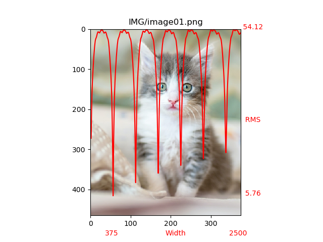
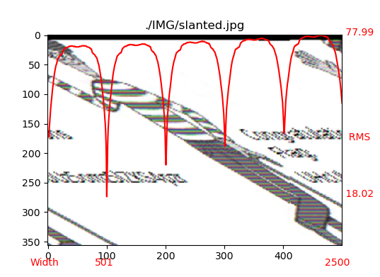
3. Results

A set of images were selected to represent different size and content. A few are shown here with their corresponding curve of RMS difference versus width. We can distinguish a photography of a cat, a synthetic composition with small graphics and text, a slanted picture with text and a chessboard (with a periodic pattern).

These examples show the sharpness of the RMS peaks and the rather large immunity of the global minimum when compared to other widths which are not multiple of the correct width. As expected we notice the progressive increase of local minima corresponding to the correct width multiples.

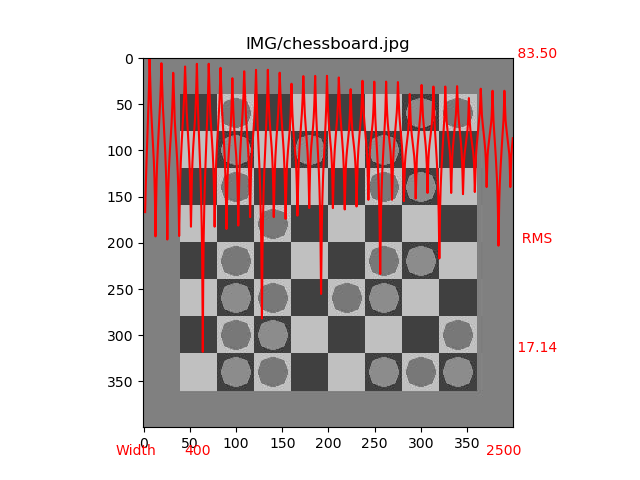
Several images with superimposed RMS vs width curves.

4. Possible improvements

Several ideas can be used to further speedup processing, if needed.

The number of visited pixels can be reduced by skipping some pixels on rows, and skipping some rows.

The number of evaluated widths can be restricted by heuristics when having an a priori knowledge of the image width or the image size ratio or thanks to the number of pixels. It can also be reduced by first considering a rough search (RMS curves tend to be smooth) and refine the obtained rough candidate for a few neighboring width values. Observing the RMS curves, a gradient descent solution should result in an important speedup by only considering a few widths. The property of local minima at multiple values of the original width can also lead to further optimisation or confirmation.

If the objective is a really fast implementation, an interesting idea would be to consider a few pairs of neighboring rows (and possibly columns) randomly chosen all over the image.

And for difficult cases with unclear RMS curve (normally due to images with poor or periodic content), an interface could let the user evaluate widths thanks to the corresponding reconstructed images.

This blog post is licensed under CC BY-SA 4.0